
Statistical Power in Hypothesis Testing: What It Is and How to Use It?
A visual guide to statistical power, significance level, effect size, and type 1/ 2 errors


What is Statistical Power?
Statistical Power is a concept in hypothesis testing that calculates the probability of detecting a positive effect when the effect is actually positive. In my previous post, we walkthrough the procedures of conducting a hypothesis testing. And in this post, we will build upon that by introducing statistical power in hypothesis testing.
Why is Statistical Power Important?
Significance level is widely used to determine how statistically significant the hypothesis testing is. However, it only tells part of the story - try to avoid claiming there is a true effect given that no actual difference exists, based on the assumption that null hypothesis is true.
But what if we care about the “positive” side of the story—the chance of reaching the correct conclusion when the alternative hypothesis is true? That’s where statistical power comes in.
Additionally, statistical power is also crucial for determining sample size. A small sample size might give a small p-value by chance, indicating that it is less likely to be a false positive mistake. But it does not guarantee that there is enough evidence for true positive. Therefore, a desired power is usually defined before the experiments to determine the minimum sample size required to reliably detect a real effect.
For a video guide to hypothesis testing, please check out our YouTube channel 🎬:
Power & Type 1 Error & Type 2 Error
In any discussion of Statistical Power, Type 1 and Type 2 errors naturally come into play. These are fundamental statistical concepts used in hypothesis testing to evaluate how our expected outcomes align with the true outcomes.
Let’s continue to use the t-test example in my previous post “Hypothesis Testing in Python (Part 1): T-Tests Explained with Code and Examples” to illustrate these concepts.
Recap: we used one-tail two sample t-test to compare two samples of customers - customers who accepted the campaign offer and customers who rejected the campaign offer.
recency_P = df[df[’Response’]==1][’Recency’].sample(n=20, random_state=100)
recency_N = df[df[’Response’]==0][’Recency’].sample(n=20, random_state=100)
null hypothesis (H0): there is no difference in Recency between the customers who accept the offer and who don’t accept the offer - represented as the blue line.
alternative hypothesis (H1): customers who accept the offer has lower Recency compared to customers who don’t accept the offer - represented as the orange line.

Type 1 error (False Positive): If values fall within the blue area in the chart, even though they occur when null hypothesis is true, we choose to reject the null hypothesis because these values are lower than the threshold, resulting in a type 1 error. It corresponds to the significance level (typically 0.05). In other words, we accept a 5% chance of incorrectly concluding that customers who accept the offer have lower recency, even though in reality there is no true difference between the two groups.
Type 2 error (False Negative): It is the probability of rejecting the alternative hypothesis when it is actually true - so claim that there is no difference between two groups when actually difference exists. In a practical business scenario, this error could cause the marketing team to overlook a valuable campaign targeting opportunity that would deliver strong return on investment.
Statistical Power (True Positive): The probability of correctly accepting the alternative hypothesis when it is true. It is the exact opposite of Type II error (Power = 1 - Type 2 error), hence when correctly predicting that customers who accept the offer are more likely to have lower Recency compared to customers who don’t accept the offer.
How to Calculate Power?
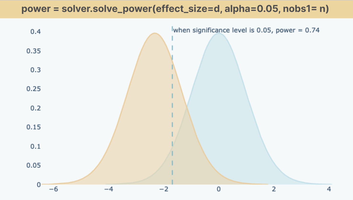
The magnitude of power is impacted by three factors: significance level, sample size and effect size. Python function solve_power() calculates the power given the values of parameters - effect_size, alpha, nobs1.
Let’s run a power analysis using the Customer Recency example above.
from statsmodels.stats.power import TTestIndPower
t_solver = TTestIndPower()
power = t_solver.solve_power(effect_size=recency_d, alpha=0.05, power=None, ratio=1, nobs1= 20, alternative=’smaller’)
significance level: we set alpha value as 0.05 which determines that the acceptable Type 1 error is 5%. alternative= ‘smaller’ is to specify the alternative hypothesis - the mean difference between two groups is smaller than 0.
sample size: nobs1 specifies the size of sample 1 (20 customers) and ratio is the number of observations in sample 2 relative to sample 1
effect size: effect_size is calculated as the difference between the mean difference relative to pooled standard deviation. For two sample t-test, we use Cohen’s d formula below to calculate the effect size. And we got 0.73. In general, 0.20, 0.50, 0.80, and 1.3 are considered as small, medium, large, and very large effect sizes.

n1 = len(recency_N)
n2 = len(recency_P)
m1, m2 = mean(recency_N), mean(recency_P)
sd1, sd2 = np.std(recency_N), np.std(recency_P)
pooled_sd = sqrt(((n1 - 1) * sd1**2 + (n2 - 1) * sd2**2) / (n1 + n2 - 2))
recency_d = (m2 - m1)/pooled_sd
How to Increase Statistical Power?
Power is positively correlated with effect size, significance level and sample size.
1. Effect Size
Larger effect size indicates a greater difference in the means relative to the pooled standard deviation. When the effect size increases, it reflects a larger observed difference between the two samples. Therefore, power increases, because there is stronger evidence that the alternative hypothesis is true.
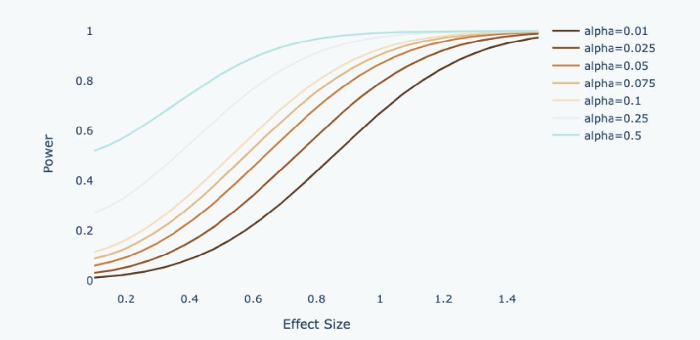
2. Significance Level & Type I Error
There is a trade-off between type 1 error and type 2 error, hence if we allow more type 1 error, power will increase accordingly. As shown in the diagram above, if we shift the threshold to reduce type 1 error, it leads to a corresponding rise in false negative errors while simultaneously diminishing statistical power. This is because if we minimize false positives, we are raising the bar and adding more constraints on what we can classify as a positive effect.
When the standard is too high, we are also reducing the probability of correctly classifying a positive effect. This means we can’t make both errors small at the same time. In practice, it is common to choose a significance level (Type I error) of 0.05 and a statistical power of 0.8, which strikes a reasonable balance in this trade-off.
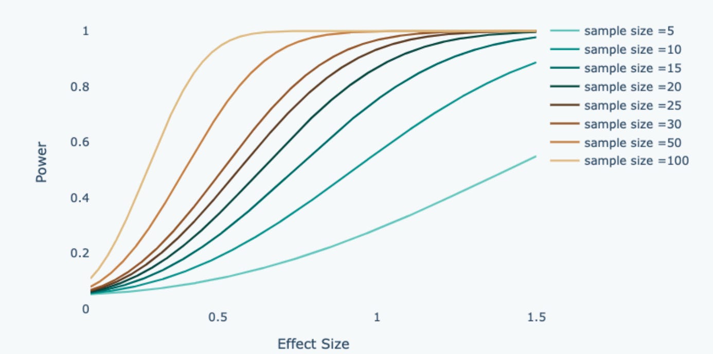
3. Sample Size
Power has a positive correlation with sample size. A large sample size brings the variance down, so the sample mean will be closer to the population mean. As a result, when we observe a difference in the sample mean, it is less likely to occur by chance.
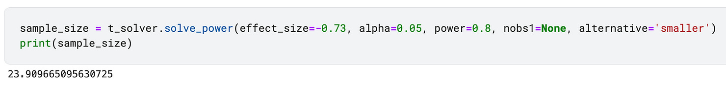
In hypothesis testing, we derive the required sample size given the desired power using the code below. For this example, it is required to have around 24 customers in each sample group to run a t-test with a power of 0.8.
Please leave a comment on this post to let me know which topics you’d like me to cover next.
Thanks for reaching so far! This post is public so feel free to share it.
Take Home Message
In this article, we introduce a statistics concept - Power, and answer some questions related to Power.
What is Statistical Power? - Power is related to Type 1 error and Type 2 error
Why we use Statistical Power? - Power can be used to determine sample size
How to calculate Power? - Power is calculated from effect size, significance level and sample size.
