
Data Science 101: Top 6 Machine Learning Algorithms for Classification
A visual guide to logistic regression, decision trees, random forests, and more ...

Three Types of Machine Learning Algorithms
The easiest way to distinguish a supervised learning and unsupervised learning is to see whether the data is labelled or not.
Supervised learning learns a function to make prediction of a defined label based on the input data. It can be either classifying data into a category (classification problem) or forecasting an outcome (regression algorithms).
Unsupervised learning reveals the underlying pattern in the dataset that are not explicitly presented, which can discover the similarity of data points (clustering algorithms) or uncover hidden relationships of variables (association rule algorithms) …
Reinforcement learning is another type of machine learning, where the agents learn to take actions based on its interaction with the environment, with the aim to maximize rewards. It is most similar to the learning process of human, following a trial-and-error approach.
Check our latest video on how to choose between two leading cloud platforms AWS and Azure for your machine learning project.
Classification vs Regression
Supervised learning can be furthered categorized into classification and regression algorithms. Classification model identifies which category an object belongs to whereas regression model predicts a continuous output.
Sometimes there is an ambiguous line between classification algorithms and regression algorithms. Many algorithms can be used for both classification and regression, and classification is just regression model with a threshold applied. When the number is higher than the threshold it is classified as true while lower classified as false.
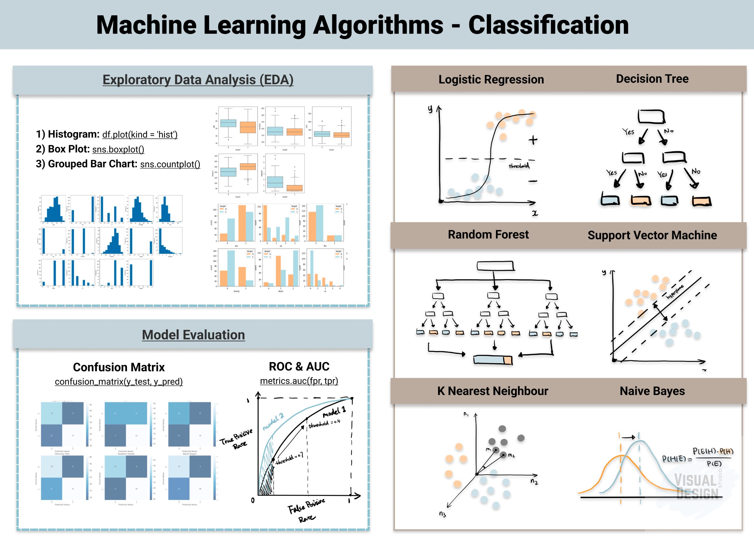
In this article, we will discuss top 6 machine learning algorithms for classification problems, including: logistic regression, decision tree, random forest, support vector machine, k nearest neighbour and naive bayes. I summarized the theory behind each as well as how to implement each using python.
For a video guide to these algorithms, please check out our YouTube channel 🎬:
Comment down below what other topics you are interested in.
1. Logistic Regression
")
Logistic regression uses sigmoid function above to return the probability of a label. It is widely used when the classification problem is binary – true or false, win or lose, positive or negative …
The sigmoid function generates a probability output. By comparing the probability with a pre-defined threshold, the object is assigned to a label accordingly.
Below is the code snippet for a default logistic regression and the common hyperparameters to experiment on – see which combinations bring the best result.
from sklearn.linear_model import LogisticRegression
reg = LogisticRegression()
reg.fit(X_train, y_train)
y_pred = reg.predict(X_test)
logistic regression common hyperparameters: penalty, max_iter, C, solver
2. Decision Tree
")
Decision tree builds tree branches in a hierarchy approach and each branch can be considered as an if-else statement. The branches develop by partitioning the dataset into subsets based on most important features. Final classification happens at the leaves of the decision tree.
from sklearn.tree import DecisionTreeClassifier
dtc = DecisionTreeClassifier()
dtc.fit(X_train, y_train)
y_pred = dtc.predict(X_test)
decision tree common hyperparameters: criterion, max_depth, min_samples_split, min_samples_leaf; max_features
3. Random Forest
")
As the name suggests, random forest is a collection of decision trees. It is a common type of ensemble methods which aggregate results from multiple predictors. Random forest additionally utilizes bagging technique to train each tree on a bootstrap sample (random sampling with replacement) of the original dataset and often on a random subset of features. Then it takes the majority vote from these trees as the final output. Compared to decision tree, it has better generalization but less interpretable, because of more layers added to the model.
from sklearn.ensemble import RandomForestClassifier
rfc = RandomForestClassifier()
rfc.fit(X_train, y_train)
y_pred = rfc.predict(X_test)
random forest common hyperparameters: n_estimators, max_features, max_depth, min_samples_split, min_samples_leaf, boostrap
4. Support Vector Machine (SVM)
")
Support vector machine finds the best way to classify the data based on the position in relation to a border between positive class and negative class. This border is known as the hyperplane which maximize the distance between closest points of different classes (i.e. support vectors). Similar to decision tree and random forest, support vector machine can be used in both classification and regression, SVC (support vector classifier) is for classification problem.
from sklearn.svm import SVC
svc = SVC()
svc.fit(X_train, y_train)
y_pred = svc.predict(X_test)
support vector machine common hyperparameters: c, kernel, gamma
5. K-Nearest Neighbour (KNN)
")
You can think of k nearest neighbour algorithm as representing each data point in a n dimensional space – which is defined by n features. And it calculates the distance between one point to another, then assign the label of unobserved data based on the labels of nearest observed data points. KNN can also be used for building recommendation system, check out my article on “Collaborative Filtering for Movie Recommendation“ if you are interested in this topic.
from sklearn.neighbors import KNeighborsClassifier
knn = KNeighborsClassifier()
knn.fit(X_train, y_train)
y_pred = knn.predict(X_test)
KNN common hyperparameters: n_neighbors, weights, leaf_size, p
6. Naive Bayes
")
Naive Bayes is based on Bayes’ Theorem – an approach to calculate conditional probability based on prior knowledge, and the naive assumption that each feature is independent to each other. The biggest advantage of Naive Bayes is that, while most machine learning algorithms rely on large amount of training data, it performs relatively well even when the training data size is small. Gaussian Naive Bayes is a type of Naive Bayes classifier that follows the normal distribution.
from sklearn.naive_bayes import GaussianNB
gnb = GaussianNB()
gnb.fit(X_train, y_train)
y_pred = gnb.predict(X_test)
gaussian naive bayes common hyperparameters: priors, var_smoothing
Now that you understand the 6 core classification algorithms, it’s time to put them into practice! In Part 2, we’ll walk through building a complete classification model pipeline using the Heart Disease UCI dataset. You’ll learn how to:
• Load and explore your dataset
• Perform exploratory data analysis (EDA)
• Split data into training and testing sets
• Create a model pipeline to compare all algorithms
• Evaluate model performance using accuracy, ROC/AUC, and confusion matrices

